
« I plan to add a few graphics, code snippets, and trim the code posted at the bottom, but I just haven’t gotten around to it. I wrote the bulk of this about two weeks ago now and just haven’t gotten around to finishing it. I’ll update this post when I can, but for now, I’m just going to publish since I have no time to clean it up. I’ll remove this message when I’ve made the post all nice and pretty (probably never).»
The other day I learned about a game Lewis Carol invented where you make “word ladders” or “word bridges.” The idea is you pick two words, and try to get from one to the other by using a chain of valid words where each word in the chain differs from the previous word by a single letter. Here’s an example:
| WORD |
| CORD |
| CORED |
| CORDED |
| CODDED |
| RODDED |
| RIDDED |
| RIDGED |
| RIDGE |
| BRIDGE |
I immediately thought making a word bridge generator would be a fun little challenge to program, and it turned out to be a slightly more difficult problem than I’d anticipated. Let’s start by formalizing this game and we’ll work our way up to what specifically makes this challenging.
Word Similarity
For our purposes, two words are similar if you can get from one word to another by “changing a letter.” This change can be an insertion (CORD->CORED), a deletion (RIDGED->RIDGE), or a substitution (WORD->CORD). This is a pretty useful similarity metric and is something of a go-to tool for a lot of natural language processing tasks: it’s called “edit distance” or “levenshtein distance” where the “distance” is the minimum number of edits to transform one word into the other, so if edit_distance(w1, w2) = 0, then w1 and w2 are the identical. Note, it’s the MINIMUM number of edits. Edit distance calculation does not need to be edits-via-valid-words like I demonstrated above, so although I was able to transform WORD into BRIDGE with 9 edits, the edit distance between these two words is actually 5:
| WORD | ||||
| WRD | – | del | ||
| BRD | – | sub | ||
| BRID | – | ins | ||
| BRIDG | – | ins | ||
| BRIDGE | – | ins |
The edit distance algorithm is a pretty neat little implementation of dynamic programming, but luckily I don’t need to build it up from scratch: python’s natural language toolkit has it built-in (be careful, it’s case sensitive):
from nltk import edit_distance
edit_distance('WORD','BRIDGE')
edit_distance('WORD','bridge')
GRAPH TRAVERSAL
In the context of this problem, we can think of our word list (i.e. the English dictionary) as an undirected graph where the nodes are words and similar words are connected. Using this formulation of the problem, a word bridge is a path between two nodes. There are several path finding algorithms available to us, but I’m only going to talk about two of the more basic ones: depth-first search (DFS) and breadth-first search (BFS).
Depth-First Search

DFS essentially goes as far along a particular branch as it can from a start node until it reaches a “terminal node” (can’t go any further) or a “cycle” (found itself back where it had already explored) and then it backtracks, doing the same thing along all the unexplored paths. If you think of a tree climber trying to map out a tree, it would be like them climbing up the trunk until they reached a fork, and then following that branch in the same direction all the way out until it reached a leaf, then working backwards to the last fork it passed, and then going forwards again until it hit a leaf, and so on.
Breadth-First Search
On the other hand, BFS looks at the graph in terms of layers. BFS first gets all the child nodes of the starting node, so now the furthest nodes are 1 edge from the start. Then it does the same thing for those children, so the furthest nodes in our searched subgraph are 2 edges away, and so on. A good visualization for this projection is a really contagious virus spreading through a population. First, people in immediate contact with patient zero get sick. Then everyone those people are in immediate contact with get sick, and so on. Replace “person” with “node” and “sick” with searched, and that’s BFS.
If we use DFS to traverse this graph, will we find the word bridge (assuming one exists, since a path does not exist between all nodes in our graph) eventually, but a) there’s no guarantee it will be the shortest path, and b) how long it takes really depends on the order of nodes in our graph, which is sort of silly. BFS will necessarily find the shortest path for us: given that we’ve searched to a depth of N edges and not found a path, we know there cannot be word bridge of length N from our start word to our target word. Therefore, if we reach our target word on the N+1 iteration of BFS, we know that the shortest path is N+1 edits. It’s possible that there are multiple “shortest paths,” but we’ll stop when we reach the first one we see.
THE BOTTLENECK
Here’s a not-so-obvious question: what part of this problem is going to cause us the biggest problems? Edit distance? The graph search? The real problem here is scale, the sheer size of the word list. Once we have everything set up, traversing the graph will be fairly easy, but building up the network will take some time.
To find a path between two arbitrary words, we need a reasonably robust dictionary. The one I had on hand for this project was 83,667 words. We need to convert this dictionary into a network. Conceptually, we do this with a similarity matrix. We take all the words in the dictionary and put all of them on each axis. For each cell in the matrix, we populate the value with the edit distance between the two words that correspond with that cell. Since we’re only concerned with entries that had edit distance “1,” we can set every other value in the matrix to zero. This reduces our similarity matrix to an adjacency matrix, describing which nodes in the graph share an edge.

Obviously, implementing this in an array structure would be wildly inefficient. Such a matrix would need to be 83,667 x 83,667, or 7,000,166,889 cells, and presumably most of them will be 0’s. If we allocate a byte to each cell in the array, this would take up 7 GB in memory. In actuality, elements of a list are allocated 4 bytes each with additional 36 bytes allocated for the list itself.
>>>import sys
>>>sys.getsizeof([])
36
>>>sys.getsizeof([1])
40
>>>sys.getsizeof([1,2])
44
Therefore, if our array is implemented as a list of lists (there are other options, such as a pandas dataframe or a numpy array, but this is the naive solution), the array would take up:
\[36 * (83,667+1) + 4 * 83,667^2 = 28,003,679,604 \text{ bytes} = 28 \text{ GB}\]
I certainly don’t have 28 GB of RAM. We’re going to need a “sparse” data structure instead, one where we get to keep the ones but can ignore the zeros. The simple solution here in python is a dictionary (which is basically just a hash table). For each word in our word list, find all similar words. In our python dictionary, the key is the searched word and the collection of matches will be our value (as a list, set, tuple…whatever).
# The adjacency matrix for the graph above converted into a sparser
# dictionary representation
## MATRIX FORM: 6 X 6 = 36 Elements
## SPARSE FORM: 18 elements
{'A':['B','C','D','E']
,'B':['A','D','E']
,'C':['A','F']
,'D':['A','B','F']
,'E':['A','B','F']
,'F':['C','D','E']
}
HEURISTICS
We’re not quite there yet. For each word, we need to look over the entire dictionary. This means our code scales with \(n^2\) (where \(n\) is the number of words in our wordlist), which sucks. Even without that knowledge, you can try the code out with this naive search and you’ll see, it will search like 20-100 words a minute. We have 83,667 words of varying size to get through before we’ve processed the graph we need for this problem, so we’ve got to come up with some tricks to make this faster.
One thing we can do is try to limit the number of words we run edit_distance() on. This function is reasonably fast, but it’s not as fast as a letter-by-letter comparison because it needs to build a matrix and do a bunch of calculations. For two words to have edit distance = 1, they can only differ by one letter. So we can compare the two letter prefix of our search word against every word in the dictionary and skip all the words whose prefixes differ by two letters. BAM! Way faster. But on my computer, this code will still take way too long to run. So let’s do the sae thing looking at suffixes. Even faster! I can’t remember, but I think at this point the estimated total run time for my code was 4 hours. Tolerable, but I’m impatient.
The problem is that although we no longer need to look at every letter of every word during a single pass, we still need to look at every word in the dictionary. But we can use the prefix/suffix heurstic we just came up with to significantly reduce the size of the seach space during any given pass though.
DIVIDE AND CONQUER

The classic divide and conquer algorithm is binary search. Consider a sorted list of numbers and some random number within the range of this list. You want to figure out where this number goes. The naive solution is called bubble sort: start at the top of the list, compare your number against that number, if yours is bigger, move to the next item. Do this until you find your number’s spot in the order. At worst, you have to look through every number in the list. For any given problem, bubble sort is almost always the wrong algorithm.

The idea behind binary search is because we know the list is already ordered, we can throw away half the list each time. Let’s say the list you’re given is 100 numbers. Jump to the middle and compare. Say your number is smaller: we don’t need to consider the top 50 numbers at all now. Now jump to the 25th number. Bigger or smaller? Throw away the other 12. And so on. In a list of 100 numbers, binary search will find the position of your random number in at most 7 steps (\(log_2(100)\)). That’s quite an improvement from bubble sort’s 100 steps.
OVERLAPPING SUBPROBLEMS
Binary search isn’t really applicable to our problem, but we can still discount a signficant amount of the search space if we appropriately pre-process our word list. As we discovered above, we can divide the word list into 3 groups relative to our target word: both two-letter affixes match, prefix matches and/or suffix matches, or neither affix matches. There are a limited number of prefixes and suffixes in our word list, so if we’re searching a word that has the same affix we’ve already searched, we’re unnecessarily repeating work. This is what’s known as an overlapping subproblem, and wherever you can identify one you can make your code faster. Oftentimes a lot faster.
We’re going to handle this affix problem by grouping the words by prefix and suffix. In other words, we’re going to build two search indexes: an index on prefix and an index on suffix. I did this using a dictionary where the affix is the key and the matching words are the values.
def build_index(words, n_letters=2, left=True, verbose=True):
    n=n_letters
    res={}
    for w in words:
        if left:
            ix = w[:n]
        else:
            ix = w[(-1)*n:]
        d = res.get(ix, [])
        d.append(w)
        res[ix] = d
    return res

>>> build_index(words)

{'AA':
['AA',
 'AAH',
 'AAHED',
 'AAHING',
 'AAHS',
 'AAL',
 'AALII',
 'AALIIS',
 'AALS',
 'AARDVARK',
 'AARDWOLF',
 'AARGH',
 'AARRGH',
 'AARRGHH',
 'AAS',
 'AASVOGEL']
,'AB':
['AB',
 'ABA',
 'ABACA',
 'ABACAS',
 'ABACI',
 'ABACK',
 'ABACUS',
 'ABACUSES',
...
 'ZYMOSES',
 'ZYMOSIS',
 'ZYMOTIC',
 'ZYMURGY',
 'ZYZZYVA',
 'ZYZZYVAS']
,'ZZ':
['ZZZ']}
This significantly speeds up our code, but if you watch the code run, it seems to speed up and slow down in bursts. This isn’t because your RAM is wonky. This is because the elements in our indexes aren’t evenly distributed. Specifically, two-letter prefixes are pretty evenly distributed, but two letter-suffixes are not.
To remedy this we’re going to use a three-letter index. An unfortunate result of my index implementation is that words that are smaller than the index size (here two letter words) don’t get considered when looking up words of size greater than or equal to the index. So although “AH” and “AAH” are similar, they’re contained in separate indexes with no overlap, so when I search for words similar to “AA” I’ll get “AT” but not “AAH”, and similarly when I look for words similar to “AAH” I’ll get “AAHS” but not “AA” or “AH.” This isn’t pefect, but I stronglly suspect the effect on the final product is negligible. I could just use a separate index size for the two prefixes, but this was simpler to code and it only just occured to me I could use a two-letter index on the left and a three-letter index on the right. So sue me. I regret nothing. The three letter index is faster anyway.
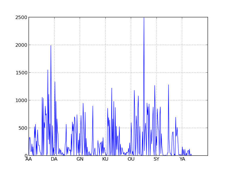
## Most Common suffixes: two letters
# ES 6810
# ED 6792
# ER 5296
# NG 4222
# RS 3480
# TS 2332
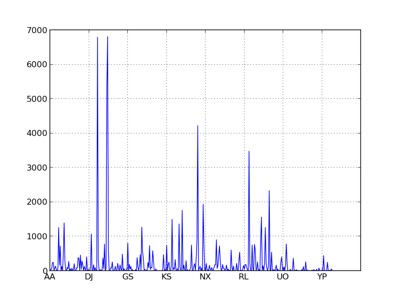
## Most Common suffixes:three letters
# ING 4062
# ERS 2743
# IER 1142
# EST 1035
# TED 1014
# IES 985
# NB: The top two three-letter suffixes combined comprise about
# the same amount of the wordlist as the top two most popular
# two-letter suffixes separately, and the rest of the suffixes
# are pretty uniformly distributed.
If you look at the X axis of the histograms below for the three letter indices you’ll notice that two letter words are segregated into their own buckets. If we made similar histograms for indices of four or five letters, these buckets would manifest as an unusual density on the far left of the graph.
With our indexes in place, we can now generate our similarity network in a reasonable amount of time: about 90 minutes on my computer.
def build_wordnet(wordlist, max_dist=1, index_size=None):
    """
    Returns a word similarity network (as a dict) where similarity is
    measured as edit_distance(word1,word2) <= max_dist. This implementation doesn't properly account for words smaller than the index size. index_size defaults to max_dist+1, but you should check the distribution of prefixes/affixes in your wordlist to judge. In an 80K dictionary, I found a 3 letter index to be suitable, although this did result in the isolation of two letter words from the major component(s) of the network. """ if index_size is None: index_size = max_dist + 1 if verbose: print "Building right index..." R_ix = build_index(wordlist, n_letters=index_size, left=False) if verbose: print "Building left index..." L_ix = build_index(wordlist, n_letters=index_size, left=True) def check_index(j, affix, index, left=True): right = not left for k in index[affix]: if abs(len(j)-len(k))>max_dist:
                continue
            if right and edit_distance(j[-1*index_size:], k[-1*index_size:]) > max_dist:
                continue
            if left and edit_distance(j[:index_size], k[:index_size]) > max_dist:
                continue
            if j == k:
                continue
            if edit_distance(j,k) <= max_dist:
                similarity_network[j].update([k])

    similarity_network = {}
    n=0
    start = time.time()
    now = 0
    last = 0
    for j in wordlist:
        similarity_network[j]=set()
        prefix = j[:index_size]
        suffix = j[-1*index_size:]
        check_index(j,suffix, R_ix, left=False)
        check_index(j,prefix, L_ix, left=True)

        if verbose:
            n+=1
            now = int(time.time() - start)/60
            if now%5 == 0 and now == last+1:
                print n, int(time.time() - start)/60
            last = now
    return similarity_network
At this point you should really think about saving your result so you don’t have to wait 90 minutes every time you want to play with this tool we’re building (i.e. we should only ever have to run these calculations once). I recommend pickling the dictionary to a file.
import cPickle

datafile = 'similarity_matrix.dat'

f=open(datafile,'wb')
p = cPickle.Pickler(f)
g = build_wordnet(words)
p.dump(g)
f.close()
NETWORKS
Now that we’ve got the structure in place, we’re ready to find some word bridges! When I first started this project, I tweaked a recipe I found online for my BFS function. It gave me results, but it was messy so I’ll spare you my code. Because we’re working with a graph, we can take advantage of special graph libraries. There are several options in python, one of which is igraph which I’ve played with a little in R and it’s fine. After some googling around, I got the impression that the preference for python is generally the networkx library, so I decided to go with that.
All we have left to do is convert our graph into a networkx.Graph object, and call the networkx path search algorithm.
import networkx as nx
net = nx.Graph()
net.add_nodes_from(words)
for k,v in g.iteritems():
    for v_i in v:
        net.add_edge(k,vi)

w1 = raw_input("Start Word: ")
w2 = raw_input("End Word:   ")
nx.shortest_path(g, w1, w2)   # BAM! Don't need to reinvent the motherfucking wheel.
Really, we could have just used this data structure from the start when we were building the network up, but the dictionary worked just fine, the conversion step is still fast, I strongly suspect the native dict pickles to a smaller file than an nx.Graph would (feel free to prove it to yourself), and it was also a better pedagogical tool. Moreover, networkx graphs are dictionary-like, so the idea is still the same.
MAKING IT BETTER: OOP
A feature we’re lacking here is the ability to add missing words. After playing with this a little I’ve found that the word list I started with is short a few words, and doesn’t contain any proper nouns (preventing me from using my own name in word bridges, for example). In the current implementation, to add a single word I would need to rebuild the whole network. I could build in a new function that adds a word to the graph, but I’d want to add this word into indexes too. This is getting complicated. But if I rebuild my tools using OOP principles, this feature will be pretty simple to add and I can reuse most of my existing code (by wrapping several things that currently appear in loops as methods). There are two kinds of entities we’re going to want to represent: indexes, and word networks.
class Index(object):
    '''
    Container class for wordbridge index, which gets stored as a dict
    in the index attribute. affix
    '''
    def __init__(self, index_size=2, left=True):
        self.index_size = index_size
        self.left = left
        self.index = {}
        self._check_if_word_in_index = False
    def in_index(self, word):
        try:
            for w in self.index[self.get_affix(word)]:
                if w==word:
                    return True
        except:
            pass
        return False
    def get_affix(self, word):
        n = self.index_size
        if self.left:
            ix = word[:n]
        else:
            ix = word[(-1)*n:]
        return ix
    def add_word(self, word):
        if self._check_if_word_in_index:
            if in_index(word):
                return
        ix = self.get_affix(word)
        d = self.index.get(ix, [])
        d.append(word)
        self.index[ix] = d
        #self.words.append(word)
    def add_words(self, words):
        if type(words) in [type(()),type([]), type(set())]:
            for w in words:
                self.add_word(w)
        elif type(words) == type(''):
            self.add_word(words)
        else:
            # This should really be an error
            return "Invalid input type"

class Wordbridge(object):
    def __init__(self, words=None, wordslist_filepath=None):
        self.g = nx.Graph()
        self.indexes = []
        self.words = set()
        if type(wordslist_filepath) == type(''):
            self.seed_words_from_file(wordslist_filepath)
        if words:
            self.seed_words(words)
    def graph_from_dict(self, net_dict):
        for k,v in net_dict.iteritems():
            for v_i in v:
                self.g.add_edge(k,v_i)
        self.words.update(net_dict.keys())
    def update_indexes(self, word):
        for ix in self.indexes:
            ix.add_word(word)
    def add_word(self, word):
        w = word.upper()
        try:
            _ = self.g.node(w) # check if node is in graph
        except:
            self.update_indexes(w)
            self.g.add_node(w)
            self.check_indexes(w)
    def add_index(self, index_size, left=True):
        '''
        Creates a new index, stored in Wordnet.indexes list"
        '''
        ix = Index(index_size, left)
        ix.add_words(self.words)
        self.indexes.append(ix)
    def seed_words(self, words):
        self.words.update(words)
        self.g.add_nodes_from(self.words)
    def seed_words_from_file(self,path):
        with open(path) as f:
            word_list = f.read().split()
        self.seed_words(word_list)
    def check_indexes(self, j, max_dist=1):
        '''
        Adds a word to the graph
        '''
        candidates = set()
        n = max_dist+2
        for ix in self.indexes:
            right = not ix.left
            left = ix.left
            affix = ix.get_affix(j)
            candidates.update(ix.index[affix])
        for k in candidates:
            if abs(len(j)-len(k))>max_dist:
                continue
            # this is sort of redundant because of the index design, but probably helps a tick.
            if edit_distance(j[-1*n:], k[-1*n:]) + edit_distance(j[:n], k[:n]) > max_dist:
                continue
            if j == k:
                continue
            if edit_distance(j,k) <= max_dist:
                #similarity_network[j].update([k])
                self.g.add_edge(j,k)
    def build_network(self, verbose=False):
        n=0
        start = time.time()
        now = 0
        last = 0
        for j in wordlist:
            check_indexes(j)
            if verbose:
                n+=1
                now = int(time.time() - start)/60
                if now%5 == 0 and now == last+1:
                    print n, int(time.time() - start)/60
                last = now
    def wordbridge(self, w1, w2):
        try:
            return nx.shortest_path(self.g, w1.upper(), w2.upper())
        except: # NetworkXNoPath error
            return "No path between %s and %s" % (w1, w2)